Project
I trained tiny LLMs on Shakespeare
smollms is my tiny architecture lab for understanding dense attention, recurrence, sparse selection, compressed memory, and MoE without pretending I have a GPU cluster.
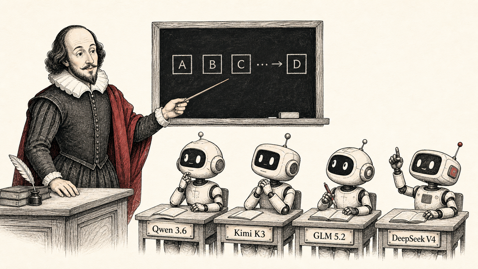
I have been reading about all these new LLM architectures for a while now. Kimi has recurrence and latent experts. GLM has token selection. DeepSeek has compressed memory and MoE. Every paper makes it sound very obvious once you finish reading it.
Then I open the actual implementation and suddenly there are twenty things happening at once. A new attention mechanism, a router, a cache, some kernel trick, a training recipe that needs a hundred GPUs, and a result table that is impossible to reproduce from my laptop.
So I made smollms.
It is a tiny, inspectable language-model lab. I trained four small decoder families on Tiny Shakespeare, character by character. Not because character-level Shakespeare is the future of AI, obviously. It is because the task is small enough that I can change one thing, run it again, and understand what actually moved.
The whole experiment runs on CPU. Every model uses the same 65-character vocabulary, 64-character context window, four layers, width 128, batch size 32, 2,000 update steps, and seed 1337. That gave me a shared little universe where I could stop hand-waving and start comparing things.
The important boundary is simple: these are toy versions of ideas from Qwen, Kimi, GLM, and DeepSeek. I am trying to learn the mechanisms, not claim that I reproduced the actual models.
i started with a boring transformer on purpose
Before I touched anything interesting, I built a normal dense decoder.
Characters become token IDs. Token IDs become vectors. Four Transformer blocks repeatedly do two jobs: attention lets a character read earlier characters, then a SwiGLU MLP changes the features at that position. RMSNorm keeps the residual stream stable, RoPE gives attention position information, and the input embedding is tied to the final output head.
characters -> token ids -> embeddings
  -> [RMSNorm -> causal attention -> residual add]
  -> [RMSNorm -> SwiGLU -> residual add] x 4
  -> RMSNorm -> next-character logits
This is the control. It is not glamorous, but it gets to look at all earlier characters directly and has very few moving parts. If a fancy branch cannot beat this setup, I should not get to call it fancy. I should call it worse.
I also made each run leave receipts behind. A folder under runs/ stores the exact command arguments, model configuration, corpus fingerprint, losses, generated sample, plot, summary, and checkpoint. That turned out to be one of the best parts of the project. A result is much less magical when I can reopen the folder and see exactly what ran.
Here is a sample from the dense control after training:
To be with me, both dignime,
Our inter you my life, by strums, maid!

QUEEN:
Your instructed her, and friends, and not the so
It is not Shakespeare, but it has discovered that Shakespeare has names, line breaks, dramatic declarations, and a vague sense that someone should probably be a queen. That is enough for this lab.
the four things i wanted to understand
I did not want one giant "best model" made from every idea I had read about. That would be impossible to learn from. Instead, each branch changes one ordinary decoder assumption.
1. dense / qwen-style: just let every token look back
The dense control is the baseline above: full causal attention plus SwiGLU. At position t, every head can score every earlier position from 0 through t, take a weighted average of their values, and pass the result onward.
It is expensive at long context lengths, but at 64 characters it is a very hard baseline to beat. It sees the whole little history and it is simple.
2. kimi-style: remember through a recurrence instead of keeping everything around
The Kimi branch has two separate ideas.
First, I replaced the dense MLP with a LatentMoE. Instead of routing directly in the full model width, a token goes down into a smaller latent space, a router selects a few specialists, an always-on shared expert handles the common work, and the output goes back up.
Then I changed the token mixer. KDA keeps one small state per attention head. Each incoming token decays the old state, predicts the current value from its key, and only writes the residual error back. Gated MLA is the other half: it still uses full causal attention, but stores smaller latent K/V representations and reconstructs them when needed.
The 1L1F schedule alternates those two kinds of layers. The all_full version keeps full attention everywhere. That gave me a clean question: does this KDA/Gated-MLA schedule help relative to the same Kimi model with full attention?
3. glm-style: decide which tokens are worth reading
The GLM experiment has a little indexer that scores the causal prefix and keeps only its top-k token positions. Normal attention then reads the selected K/V vectors.
The intuition is really nice. Instead of asking attention to look at everything, first ask a cheaper module what matters, then only read that.
For the experiment, I kept the routed MoE channel mixer fixed and changed only the token mixer: learned top-k selection versus ordinary dense attention. This mattered because otherwise I would not know whether an outcome came from the selector or the experts.
4. deepseek v4-style: keep nearby detail, compress the past
The V4 branch splits history into three parts:
completed old chunks -> learned compressed memory
partial boundary     -> raw K/V
recent local window  -> raw K/V
The partial boundary is the little detail I like most. If the local window cuts through a chunk, that chunk cannot be treated as fully compressed without losing a few tokens. Keeping the boundary raw means every old character has exactly one representation: compressed, raw boundary, or raw local context.
I also made a dense-SwiGLU version and a mixed-MoE version while keeping this attention layout fixed. The first layer uses a simple token-ID hash route; later layers use learned routed experts. Again, one question at a time: does the channel mixer help here?
then i had to make the comparisons not lie
At first I wanted to put every run in one big table and see who won. But that is kind of fake when the models have different parameter counts and do different work per token.
So I only compare controlled pairs. Same Tiny Shakespeare corpus, same seed, same optimizer, same context length, same width and depth, same steps. Change one thing. Then show parameter count and wall time next to the loss instead of hiding the bill.
This is the most important rule in the whole project. A lower loss is not the full story if it needed more parameters or five times more time to get there.
what happened
Kimi learned better, but it made me wait for it
The full-attention Kimi control ended at validation loss 1.7335. The 1L1F KDA/Gated-MLA schedule reached 1.4441.
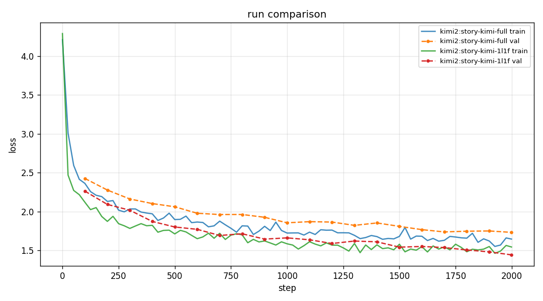
| Kimi schedule | Parameters | Validation loss | CPU wall time |
|---|---|---|---|
all_full | 387,072 | 1.7335 | 243.6 s |
1L1F | 469,888 | 1.4441 | 1,118.6 s |
That is a satisfying result because the loss actually moves a lot. It is also a good reminder that a good result can come with a very annoying tradeoff. The hybrid took 4.6x as long and has more parameters. I came away thinking: okay, recurrence and latent attention are not automatically bad ideas. But they definitely did not give me a free win.
GLM token selection lost to ordinary dense attention
This one was more useful because it was disappointing.
With the same seed and same routed-MoE setup, the GLM top-k selector got best validation loss 2.1032. Dense attention got 1.5021. Dense attention was also faster.
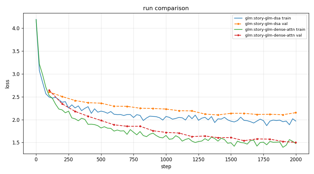
| GLM token mixer | Parameters | Best validation loss | CPU wall time |
|---|---|---|---|
| DSA top-k selector | 1,454,080 | 2.1032 | 369.7 s |
| Dense attention | 1,388,544 | 1.5021 | 253.0 s |
The selector was the thing that changed, so the result is quite direct: in this tiny 64-character setup, my selector made the model worse.
That is not a reason to say GLM-style selection is bad. It is a reason to stop blaming the experts, stop guessing, and look at the selector. Maybe learned selection needs a context long enough for selection to matter. Maybe the indexer needs more work. Maybe this particular toy is just not good enough. All of those are much better next questions than pretending the result is secretly fine because the idea sounded cool.
Also, the current implementation still builds a dense index-score matrix before taking top-k. So it teaches the selection data flow, but it does not prove any sparse-attention speedup. I will worry about kernels only when I have an experiment that actually needs them.
the V4 MoE gave me a small gain and a very visible bill
The V4 branch kept local-plus-compressed attention fixed and changed the channel mixer. The mixed MoE lowered validation loss from 1.5215 to 1.4865.
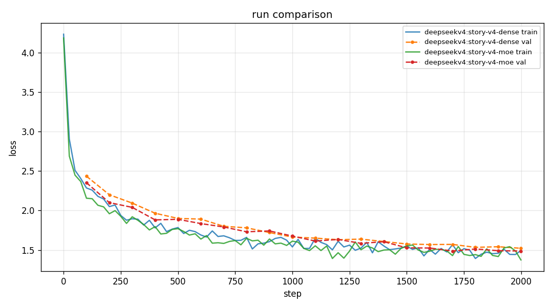
| V4 channel mixer | Parameters | Validation loss | CPU wall time |
|---|---|---|---|
| Dense SwiGLU | 833,024 | 1.5215 | 244.7 s |
| Hash-then-routed MoE | 1,289,728 | 1.4865 | 355.1 s |
The gain is real in this run, but it is small: 0.0350 validation loss. The cost is 456,704 extra parameters and about 45% more wall time.
This is exactly why I wanted the run artifacts. If I only looked at the last number, I would write "MoE wins." If I look at the full folder, I get a more honest answer: this is promising enough to repeat with more seeds, but not enough to get carried away.
the nicest part was learning what not to conclude
I thought the project would mostly teach me how attention and MoE work. It did, but it also taught me how easy it is to make an experiment say more than it should.
- A generated sample is fun, but validation loss is the signal I should compare first.
- Different parameter counts are not a footnote. They are part of the result.
- A single seed can show something interesting, but it cannot settle a general architectural question.
- "This did not help at 64 characters" is a complete and useful result. It does not need to become a dramatic verdict on an entire model family.
- The boring dense decoder is a serious baseline, not something to rush past.
Right now smollms is intentionally small enough to read. The architecture lab walks through the implementations in more detail, the results page links every measured run, and the experiment report has the full paper-style version with all the receipts.
If you want to run the same suite, it is just this:
git clone https://github.com/TarunTomar122/smollms
cd smollms
python3 -m venv .venv
source .venv/bin/activate
python -m pip install -e ".[dev]"

SEED=1337 DEVICE=cpu STEPS=2000 sh scripts/train_story_suite.sh
The next thing I want to do is not make it bigger for the sake of it. I want to repeat the interesting pairs with a couple more seeds, keep changing one block at a time, and see which explanations survive.
That feels much more fun than reading another architecture diagram and pretending I understood it.