Writing
Making a small language model slower on purpose
A quest to understand how GPUs work
Chapter 1: The question
I started with a simple question: I wanted to learn how GPUs work, how memory works in GPUs, and what CUDA is. I learned all of that, and then I wanted to put it into practice with a project.
I thought for a while about doing a project that improves the efficiency of a model or something like that, but I kept getting blocked because I didn't know enough yet. I really wanted to still do something meaningful.
That's when I flipped the switch completely. Instead of making something more efficient, I realized another way to learn about GPUs is to try and make something less efficient. The whole idea became this: take a small language model and try to make it slower on purpose.
Chapter 2: The setup
I ran the experiment on Google Colab, using the Qwen3-0.6B model, mostly because it's small and fast to iterate on. We're using a Tesla T4 GPU, which has around 14.56 GiB of VRAM, compute capability 7.5, CUDA 12.8, PyTorch 2.11.0, and Triton 3.2.0.
Triton was very new to me. I had never previously used Triton to write GPU code, so this is what the entire learning was really about. The model was loaded in FP16, generation used deterministic decoding, and everything ran with a fixed number of new tokens so the measurements were actually comparable.
First baseline numbers, before I touched anything:
| Measurement | Result |
|---|---|
| Prefill throughput | 4,171.98 tokens/s |
| 128-token end-to-end generation | 22.64 tokens/s |
| KV cache enabled | 23.07 tokens/s |
| KV cache disabled | 11.39 tokens/s |
I tried disabling the KV cache, and the output TPS dropped by almost more than half. Pretty interesting, but still basic stuff: reusing previous keys and values means you're not recomputing the whole history for every generated token.
Chapter 3: My first kernel
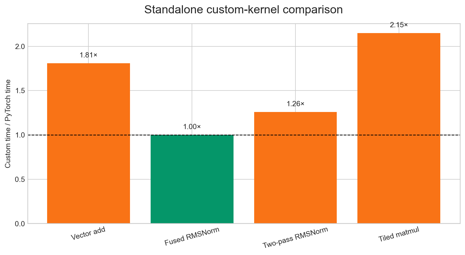
Now the time came to write my first ever kernel. I started with a very simple addition kernel and compared it against PyTorch's native addition function. My kernel ran at 0.084 ms vs PyTorch's 0.046 ms, about 1.81x slower.
The result was, of course, that my kernel was slightly worse than PyTorch's, for obvious reasons. PyTorch uses very highly efficient kernels, tiling, all of that. Mine didn't, so mine was slower. That's what we wanted, so that's a good thing.
Chapter 4: RMSNorm, and the trick of un-fusing
After that I got onto writing a kernel for RMS normalization, because the model does this in a lot of places in its pipeline. I thought if I could replace RMS norm with my own custom kernel, I could make the whole thing slower.
I wrote a fused kernel first, doing pretty much everything PyTorch's native kernel does, and apparently I didn't get much of a speed drop. That was sad, honestly, because I really wanted to drop the speed and that didn't happen. I was slightly worse, but not clearly bad, so I needed a way to deliberately make it worse.
So I un-fused it. RMS norm has two operations, normalization and scaling, and I separated them into two different sub-kernels:
- Pass 1: read
xand calculate the inverse RMS, write it back to memory - Pass 2: read from memory again, do the scaling calculation, save back
This constant read and write from memory made my kernel memory-bound, while the actual calculation was very quick. So the kernel became worse than the native one, purely because of memory traffic. That's the whole trick.
The two-pass version matched PyTorch's output within tolerance, and measured 1.26x slower overall. The gap showed up a lot more at small batch sizes:
| Rows | PyTorch | Two-pass Triton | Ratio |
|---|---|---|---|
| 1 | 0.051 ms | 0.241 ms | 4.72x |
| 512 | 0.096 ms | 0.200 ms | 2.08x |
| 4096 | 0.126 ms | 0.238 ms | 1.89x |
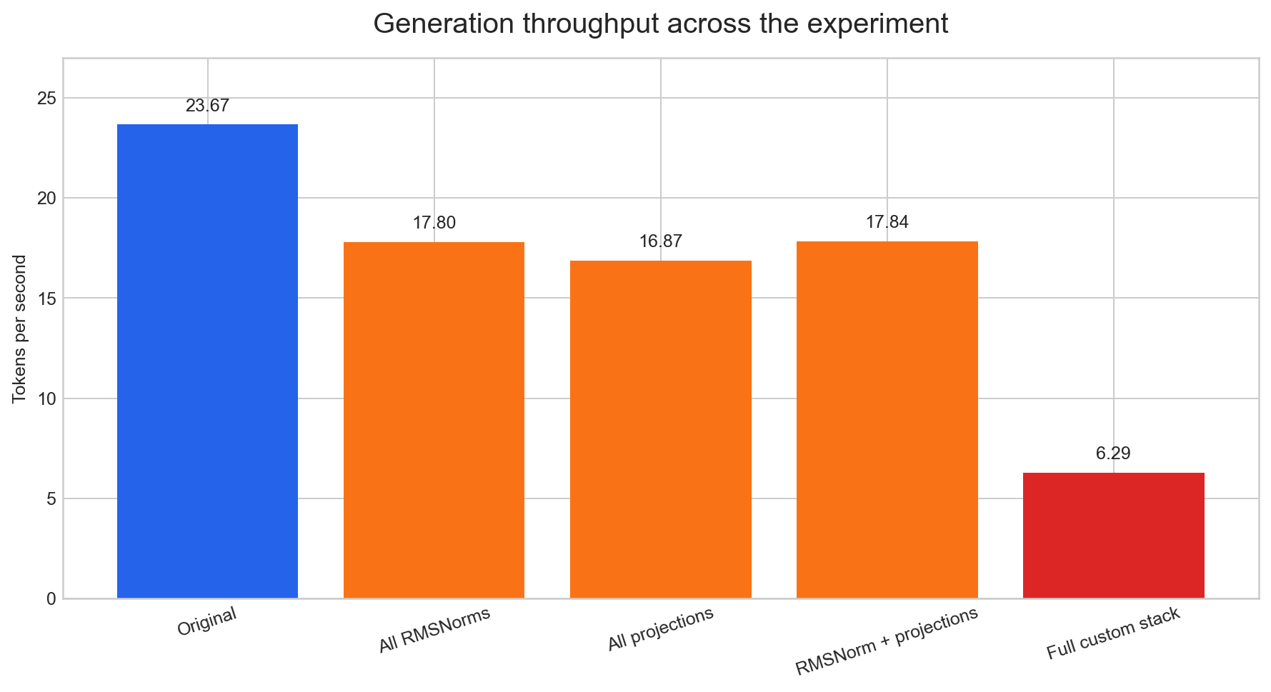
I replaced all 113 Qwen RMS norm modules with my kernel, and TPS went from 23.38 to 17.80. A good case for us.
Chapter 5: A tiled matmul, and attention projections
Next I wanted to take it to the next level, so I started writing a kernel for matrix multiplication: A[M,K] × B[K,N] = C[M,N]. Each Triton program handled one output tile, first using 64x64 output tiles and chunking the shared K dimension in blocks of 32.
I once again tested correctness first, and the output using my kernel matched PyTorch, which made me happy (max FP16 error of 0.03125). At a model-shaped input, PyTorch took 0.106 ms against Triton's 0.229 ms.
Tile size mattered a lot more than I expected. On a decode-shaped workload with one output row, sweeping BLOCK_M gave:
| BLOCK_M | Triton latency |
|---|---|
| 16 | 0.319 ms |
| 32 | 0.198 ms |
| 64 | 0.215 ms |
Then I replaced all 112 attention projections with my custom kernel and got another slowdown, going from 23 TPS down to 17 TPS this time, purely from swapping in the custom matmul. Adding the 84 MLP projections on top brought the full projection stack to 1.41x slower.
Combining all the custom projections (112 attention + 84 MLP + 1 lm_head) with the two-pass RMS norm gave:
- Original: 23.67 tokens/s
- Custom: 17.84 tokens/s, a 1.33x slowdown, purely from mathematically equivalent operations with less optimized tiling and more kernel launches.
Chapter 6: Attention, the most interesting part
The third and most interesting thing so far was attention itself, where the Q, K, V, and softmax stuff happens. I wrote a kernel that did the matrix multiplication, softmax, and scaling back, all from scratch.
To build it, I first used plain PyTorch operations inside my own kernel, just to see the shape of the problem. The actual fused SDPA was 0.149 ms, and my PyTorch-inside-my-kernel version took 0.327 ms. The difference wasn't great, but I really wanted to make it properly bad.
So I swapped in my own matmul kernel to do the actual multiplication, on a decode-shaped input:
Q: [1, 16, 1, 64]
K: [1, 16, 512, 64]
V: [1, 16, 512, 64]
This meant looping over all 16 heads, doing matmul, softmax, and giving the final output, with two matmul launches per head:
| Attention path | Latency |
|---|---|
| Fused SDPA | 0.149 ms |
| Explicit PyTorch ops | 0.327 ms |
| Triton matmul per head | 8.521 ms |
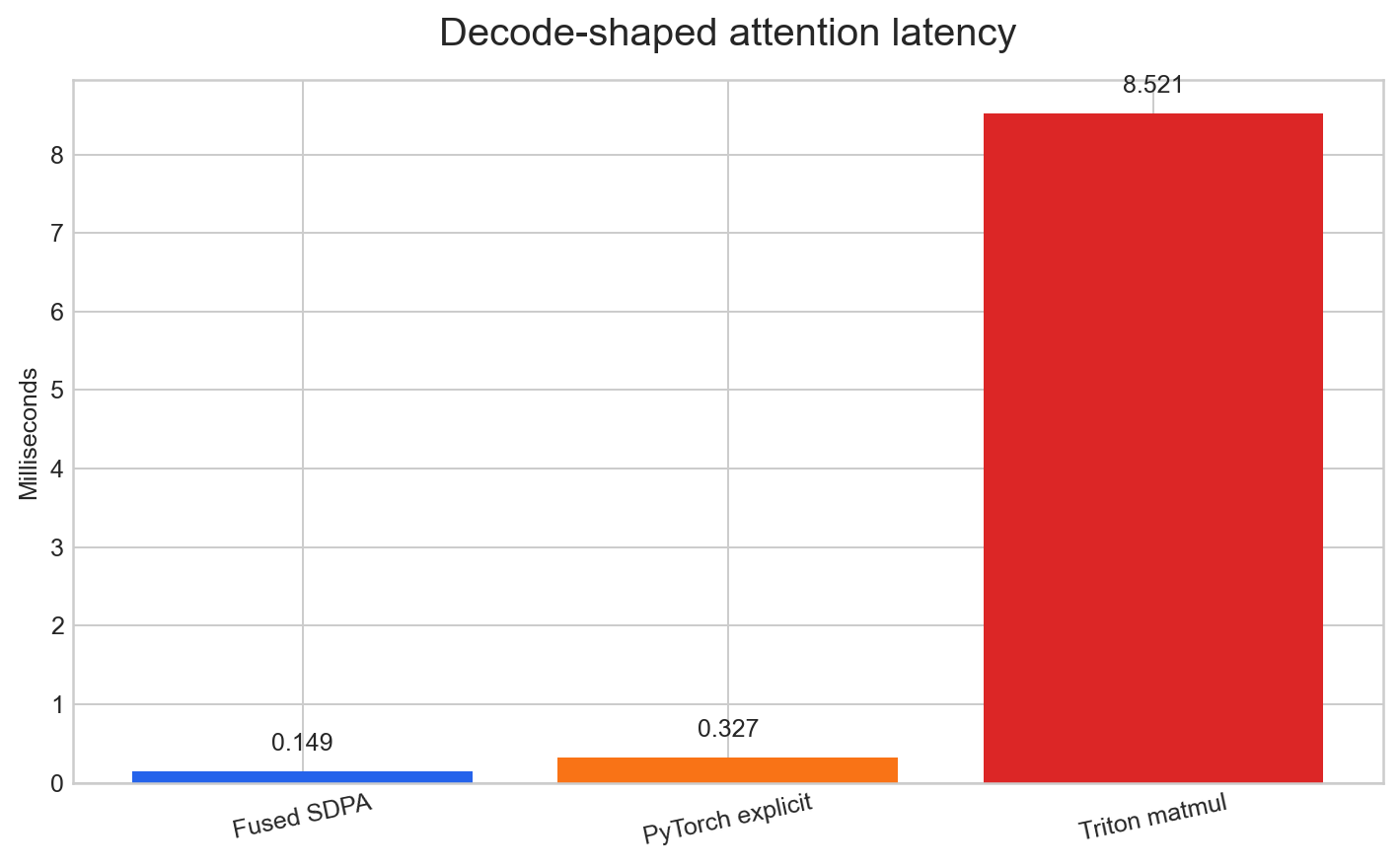
8.5 ms. This was because of the two loops going over all the batch items, doing matmul, softmax, and the final output for each one. This was a great result because it was really slow, and honestly the clearest demonstration of launch overhead in the whole project.
Chapter 7: The final stack
The final thing I did was combine all 113 RMS norms, 197 matrix multiplications, and 28 attention modules, all running my custom kernels, and benchmark it on 512 tokens.
- Original: 22.58 tokens/s
- Custom: 6.29 tokens/s
- Slowdown: 3.59x
Worth noting: the custom attention path follows a different floating-point operation order than PyTorch's fused backend, even though it matched exactly in isolated comparison. Stacked across all 28 layers, the generated tokens ended up diverging from the original model's output. That's an expected and kind of fun side effect, not a bug, just floating-point reality.
Chapter 8: Does the slowdown hold as context grows?
Then I tried it with a bunch of different context lengths, fixing generation at 32 tokens and sweeping the prompt from 128 to 1024, every custom kernel enabled.
| Context | Original | All custom | Slowdown |
|---|---|---|---|
| 128 | 23.86 tok/s | 6.12 tok/s | 3.90x |
| 256 | 24.02 tok/s | 6.16 tok/s | 3.90x |
| 512 | 23.38 tok/s | 6.37 tok/s | 3.67x |
| 1024 | 21.14 tok/s | 6.45 tok/s | 3.28x |
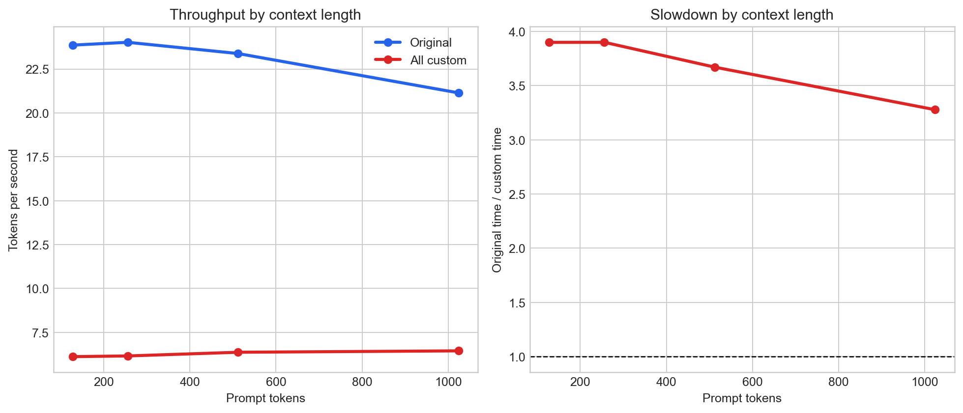
The custom kernel held the slowdown rate around 3.2x to 3.9x as the context grew, though the ratio got slightly less as context got longer. That's mostly because of the prefill part: the original model naturally slows down as context grows since its attention cost scales up too, while the custom model stays pinned near 6 tokens per second because launch overhead is the bottleneck, not the attention math itself.
What I actually learned
This experiment taught me a lot about:
- kernels
- how memory works in GPUs
- how fused and un-fused kernels work
- how Python orchestrates around a lot of small GPU operations
The biggest lesson: a mathematically correct kernel can still be a bad GPU implementation. Performance depends on workload shape, memory layout, launch count, and how much work each kernel program actually does, not just whether the math checks out.
Overall it was a great experiment, and the failure results were exactly what I was looking for.
Next up: do the opposite. Take this same baseline and optimize one kernel at a time, and see how much speed each fix actually recovers.
Byeeee!!!!